Wave Sampling
Introduction
Geographical data are generally auto-correlated, making it preferable to avoid sampling neighboring units. We introduce a new method for selecting well-spread samples from a finite spatial population with equal or unequal inclusion probabilities. The proposed method, called wave (Weakly Associated Vectors), defines the contiguity structure using dense stratification. This method precisely satisfies inclusion probabilities while providing well-spread samples. This document serves as an introduction to using the wave() function.
Data Generation
We use the meuse dataset from the sp package, described as follows:
This dataset provides locations and topsoil heavy metal concentrations, along with various soil and landscape variables recorded at observation locations in a floodplain of the river Meuse, near Stein (NL).
As explained by Grafström and Tillé (2013), we generate inclusion probabilities proportional to copper concentration, a highly spatially correlated variable.
library(sp)
library(sf)
library(sampling)
library(WaveSampling)
data("meuse")
data("meuse.riv")
meuse.riv <- meuse.riv[which(meuse.riv[,2] < 334200 & meuse.riv[,2] > 329400),]
meuse_sf <- st_as_sf(meuse, coords = c("x", "y"), crs = 28992, agr = "constant")

X <- scale(as.matrix(meuse[,1:2]))
pik <- inclusionprobabilities(meuse$copper,30)
Sample selection
We perform sample selection easily using the wave() function.
s <- wave(X,pik)
sum(s)
#> [1] 30
Data visualization
The selected sample is visualized using ggplot2.
library(ggplot2)
p <- ggplot()+
  geom_sf(data = meuse_sf,aes(size=copper),show.legend = 'point',shape = 1,stroke = 0.3)+
  geom_polygon(data = data.frame(x = meuse.riv[,1],y = meuse.riv[,2]),
               aes(x = x,y = y),
               fill = "lightskyblue2",
               colour= "grey50")+
  geom_point(data = meuse,
             aes(x = x,y = y,size = copper),
             shape = 1,
             stroke = 0.3)+
  geom_point(data = meuse[which(s == 1),],
             aes(x = x,y = y,size = copper),
             shape = 16)+
  labs(x = "Longitude",
       y = "Latitude",
       title = NULL,
       size = "Copper",
       caption = NULL)+
  scale_size(range = c(0.5, 3.5))+
  theme_minimal()
p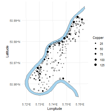
Spatial balance
Voronoï polygons
One way of measuring the spread of a sample was developed by Stevens Jr. and Olsen (2004) and then suggested by Grafström et al. (2012). It is based on the Voronoï polygons and is given by
\[B(\bf s) = \frac{1}{n}\sum_{i \in s} (v_i - 1)^2\]where \(v_i\) is equal to the sum of the inclusion probabilities inside the \(i\)th polygons and \(\bf s\) is the vector of size \(N\) with elements equal 0 or 1. This quantity is implemented in the package BalancedSampling with the function sb(). We calculate the values of the \(v_k\) with the function sb_vk.
The closer \(B(\bf s)\) is to zero, the better is the spatial balance of the sample. Graphically, we obtain the following plot.
library(sp)
library(sampling)
library(ggvoronoi)data("meuse")
data("meuse.area")
v <- sb_vk(pik,as.matrix(meuse[,1:2]),s)
meuse$v <- v
p <- p + geom_voronoi(data = meuse[which(s == 1),],
aes(x = x,y = y,fill = v),
outline =as.data.frame(meuse.area),
size = 0.1,
colour = "black")+
geom_point(data = meuse,
aes(x = x,y = y,size = copper),
shape = 1,
stroke = 0.3)+
geom_point(data = meuse[which(s == 1),],
aes(x = x,y = y,size = copper),
shape = 16)+
scale_fill_gradient2(midpoint = 1)
p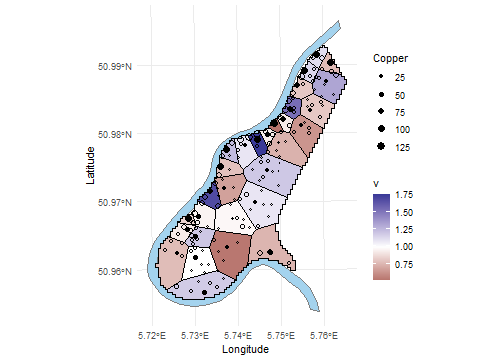
BalancedSampling::sb(pik,as.matrix(meuse[,1:2]),which(s == 1))#> [1] 0.0910097Moran index
Another way to estimate the spatial spread is developed by Tillé et al. (2018), it uses a corrected version of the traditional Moran’s \(I\) index. This estimator use spatial weights \(w_{ij}\) that indicates how a unit \(i\) is close from the unit \(j\). Such matrix is supposed to include inclusion probabilities in its computation, hence, the spatial weights matrix \(\bf W\) is generally not symmetric. The spatial balance measure is given by
\[I_B =\frac{(\bf s-\bf \bar{s}_w)^\top \bf W (\bf s-\bf \bar{s}_w)}{\sqrt{(\bf s-\bf \bar{s}_w)^\top \bf D (\bf s-\bf \bar{s}_w) (\bf s-\bf \bar{s}_w)^\top \bf B (\bf s-\bf \bar{s}_w) }},\]where \(\bf D\) is the diagonal matrix containing the \(w_i\),
\[\bf \bar{s}_w = \bf 1 \frac{\bf s^\top \bf W \bf 1}{\bf 1^\top \bf W \bf 1},\]and
\[\bf B = \bf W^\top \bf D^{-1} \bf W - \frac{\bf W^\top \bf 1\bf 1^\top \bf W}{\bf1^\top \bf W \bf 1}.\]The Moran’s \(I\) index is implemented in the function IB(). It is possible to specify your own spatial weights with the argument W. There is no natural way of defining \(\bf W\), here we propose to consider for each unit only the neighbour such that the sum of the inclusion probabilities of the stratum sum up to 1. It is implemented in the function wpik(). Another way of estimating the spatial weights is developed by Tillé et al. (2018) and use the inverse of the inclusion probabilities \(1/\pi_i\) to estimate the neighbours of the unit \(i\). It is implemented in the function wpikInv(). As explain by Tillé et al. (2018), \(w_{ii}\) is supposed to be equal to 0 for all \(i \in U\). By construction the function wpik does not return the diagonal equal to zero. So if we want to calculate the Moran’s I index with wpik, we need to subtract the diagonal of the returned matrix.
W <- wpik(X,pik)
W <- W - diag(diag(W))
IB(W,s)
#> [1] -0.4895601W1 <- wpikInv(X,pik)
IB(W1,s)#> [1] -0.4554427References
Grafström, A., Lundström, N. L. P., and Schelin, L., (2012). Spatially balanced sampling through the pivotal method, Biometrics, 68(2):514-520 DOI: https://doi.org/10.1111/j.1541-0420.2011.01699.x
Grafström, A. and Tillé, Y., Doubly balanced spatial sampling with spreading and restitution of auxiliary totals, Environmetrics, 14(2):120-131 DOI: https://doi.org/10.1002/env.2194
Stevens Jr., D.L. and Olsen, A. R. (2004), Spatially balanced sampling of natural resources. Journal of the American Statistical Association, 99(465):262-278 DOI: https://doi.org/10.1198/016214504000000250)
Tillé, Y., Dickson, M. M., Espa, G., and Giuliani, D. (2018). Measuring the spatial balance of a sample: A new measure based on Moran’s I index, Spatial Statistics, 23:182-192 DOI: https://doi.org/10.1016/j.spasta.2018.02.001